Note
Go to the end to download the full example code.
Mixture Model#
This notebook contains the code for a simple implementation of the Leaspy Mixture model on synthetic data. Before implementing the model take a look at the relevant mathematical framework in the user guide.
The following imports are required libraries for numerical computation, data manipulation, and visualization.
import os
import matplotlib.pyplot as plt
import numpy as np
import pandas as pd
import torch
import leaspy
from leaspy.io.data import Data
This toy example is part of a simulation study, carried out by Sofia Kaisaridi that will be included in an article to be submitted in a biostatistics journal. The dataset contains 1000 individuals each with 6 visits and 6 scores.
leaspy_root = os.path.dirname(leaspy.__file__)
data_path = os.path.join(leaspy_root, "datasets/data/simulated_data_for_mixture.csv")

all_data = pd.read_csv(data_path, sep=";", decimal=",")
all_data["ID"] = all_data["ID"].ffill()
all_data = all_data.set_index(["ID", "TIME"])
all_data.head()
We load the Mixture Model from the leaspy library and transform the dataset in a leaspy-compatible form with the built-in functions.
from leaspy.models import LogisticMultivariateMixtureModel

leaspy_data = Data.from_dataframe(all_data)
Then we fit a model with 3 clusters and 2 sources. Note that we have an extra argument n_clusters than the standard model that has to be specified in order for the mixture model to run.
model = LogisticMultivariateMixtureModel(
    name="multi",
    source_dimension=2,
    dimension=6,
    n_clusters=3,
    obs_models="gaussian-diagonal",
)

model.fit(leaspy_data, "mcmc_saem", seed=1312, n_iter=100, progress_bar=False)
model.summary()
Fit with `AlgorithmName.FIT_MCMC_SAEM` took: 5.99s

================================================================================
                                 Model Summary
================================================================================
Model Name: mixture_logistic
Model Type: LogisticMultivariateMixtureModel
Features (6): score_1_normalized, score_2_normalized, score_3_normalized,
    score_4_normalized, score_5_normalized, score_6_normalized
Sources (2): Source 0 (s0), Source 1 (s1)
Clusters (3): Cluster 0 (c0), Cluster 1 (c1), Cluster 2 (c2)
Observation Models: gaussian-diagonal
Neg. Log-Likelihood: -5338.2385
Parameters: 46
BIC: -93961.79
AIC: -94187.55
ICL: -93830.93

Training Metadata
--------------------------------------------------------------------------------
Algorithm: mcmc_saem
Seed: 1312
Iterations: 100

Data Context
--------------------------------------------------------------------------------
Subjects: 1000
Visits: 6000
Total Observations: 36000
Leaspy Version: 2.1.0
================================================================================

Population Parameters
--------------------------------------------------------------------------------
  betas_mean:
                          s0        s1
            b0       -0.0099    0.0054
            b1       -0.0062    0.0054
            b2        0.0372   -0.0189
            b3        0.0329   -0.0143
            b4        0.0424   -0.0385
                          c0        c1        c2
  probs               0.3247    0.4001    0.2752
                    score_1.  score_2.  score_3.  score_4.  score_5.  score_6.
  log_g_mean          0.6386    1.6792    2.2111    0.9981    0.4451   -0.0358
                    score_1.  score_2.  score_3.  score_4.  score_5.  score_6.
  log_v0_mean        -5.0169   -5.0958   -6.3110   -5.1638   -5.3070   -5.6924

Individual Parameters
--------------------------------------------------------------------------------
                          c0        c1        c2
  tau_mean           71.0264   66.0683   57.4709
                          c0        c1        c2
  tau_std            10.4716    8.8100   11.6153
                          c0        c1        c2
  xi_mean            -0.1970   -0.2768    0.6348
                          c0        c1        c2
  xi_std              0.8801    0.9058    1.0671
  sources_mean:
                          c0        c1        c2
            s0       -1.1791   -0.9338    2.7506
            s1        2.4279   -0.8996   -1.5589

Noise Model
--------------------------------------------------------------------------------
                    score_1.  score_2.  score_3.  score_4.  score_5.  score_6.
  noise_std           0.0744    0.0715    0.0370    0.0625    0.0812    0.0779

Derived Parameters (interpretable scale)
--------------------------------------------------------------------------------
                    score_1.  score_2.  score_3.  score_4.  score_5.  score_6.
  v0                  0.0066    0.0061    0.0018    0.0057    0.0050    0.0034
                    score_1.  score_2.  score_3.  score_4.  score_5.  score_6.
  p0                  0.3456    0.1572    0.0988    0.2693    0.3905    0.5090
================================================================================
First we take a look at the population parameters. With the mixture model we obtain separate values for the tau_mean, xi_mean and the sources_mean for each cluster, as well as the cluster probabilities (probs).
model.info()
================================================================================
                               Model Information
================================================================================
Statistical Model
Type: LogisticMultivariateMixtureModel
Name: mixture_logistic
Dimension: 6
Source Dimension: 2
Observation Models: gaussian-diagonal
Parameters: 46
Clusters: 3

Latent Variables
--------------------------------------------------------------------------------
  Population:
    betas                Normal(betas_mean, betas_std)
    log_g                Normal(log_g_mean, log_g_std)
    log_v0               Normal(log_v0_mean, log_v0_std)
  Individual:
    sources              MixtureNormal(sources_mean, sources_std, probs)
    tau                  MixtureNormal(tau_mean, tau_std, probs)
    xi                   MixtureNormal(xi_mean, xi_std, probs)
--------------------------------------------------------------------------------

Training Dataset
--------------------------------------------------------------------------------
Subjects: 1000
Visits: 6000
Scores (Features): 6
Total Observations: 36000
Visits per Subject: Median 6.0 [Min 6, Max 6, IQR 0.0]

Training Details
--------------------------------------------------------------------------------
Algorithm: mcmc_saem
Seed: 1312
Iterations: 100
  Burn-in: 90/100 (90%)
  Burn-out: 10
Duration: 5.992s

Hyperparameters (fixed values from the source code)
--------------------------------------------------------------------------------
  betas_std: 0.01
  log_g_std: 0.01
  log_v0_std: 0.01
  sources_std: 1.0

Leaspy Version: 2.1.0
================================================================================
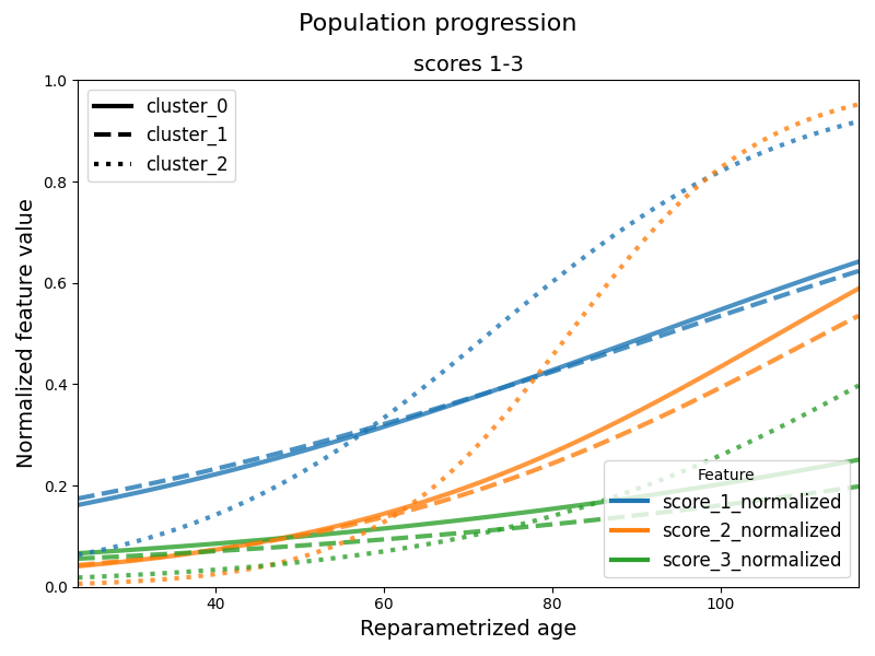
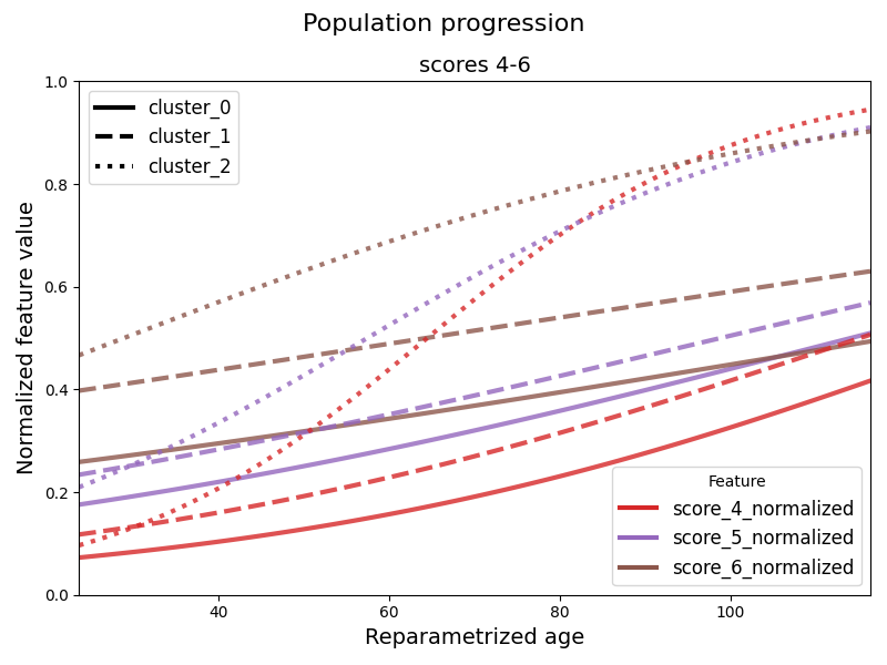
Then we can plot the average trajectory for each cluster. When having many scores the default option is to provide graphs for every three scores for readability. We can change this by providing the n_features_per_plot argument to the following function. The default option is to plot all the clusters. We can control this by providing a list of cluster indices to plot at the argument clusters.
from leaspy.io.logs.visualization.plotting import Plotting

leaspy_plotting = Plotting(model)
leaspy_plotting.average_trajectory_cluster(
    alpha=0.8,
    linewidth=3,
    figsize=(14, 6),
    n_std_left=4,
    n_std_right=5
    )
plt.show()
We can also access the individual parameters of each patient with the personalize method. Then the get_individual_probabilities method can be used to obtain the probability of each patient to belong to each cluster. The individual cluster assignment can be obtained by taking the cluster with the highest probability for each patient.
ip = model.personalize(leaspy_data, "scipy_minimize", seed=0, progress_bar=False)
ip_df = ip.to_dataframe()
ip_with_probs = model.get_individual_probabilities(ip_df)
ip_with_probs.head()
Personalize with `AlgorithmName.PERSONALIZE_SCIPY_MINIMIZE` took: 5m 4.48s
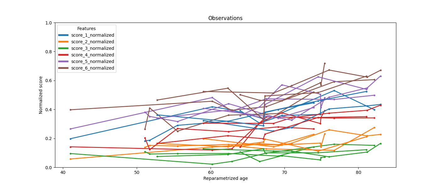
We can also plot the patient observations.
ax = leaspy_plotting.patient_observations_reparametrized(
    leaspy_data, ip_with_probs, figsize=(14, 6),
    patients_idx=['subj_1','subj_2','subj_3','subj_4','subj_5'],
)
plt.show()
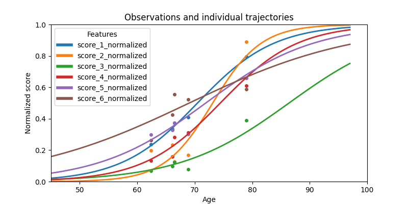
Or the patient trajectories.
ax = leaspy_plotting.patient_trajectories(
    leaspy_data,
    ip_with_probs,
    patients_idx=['subj_12']
)
ax.set_xlim(45, 100)
plt.show()
This concludes the Mixture Model example using Leaspy. We can also use these fit models to simulate new data according to the estimated parameters. This can be useful for validating the model, for generating synthetic datasets for further analysis or for generate a trajectory for a new individual given specific parameters. Let’s check this in the next example.
Total running time of the script: (5 minutes 16.401 seconds)