Note
Go to the end to download the full example code.
Personalization: Parkinson’s disease progression and inference modeling with Leaspy#
This example walks through the core Leaspy workflow on a synthetic Parkinson’s disease dataset:
Fit a shared progression model on a training cohort.
Personalize the model to new patients — estimating where each one sits on the shared disease timeline and how fast they are progressing.
Reconstruct and predict individual trajectories from those two numbers alone.
The key concept is personalization: once a model is trained, a new patient needs only a handful of visits for Leaspy to estimate their individual parameters (τ, ξ) and predict their future course.
We load a synthetic dataset of Parkinson’s patients with repeated measurements of three MDS-UPDRS motor subscores over time.
from leaspy.datasets import load_dataset
from leaspy.io.data import Data

df = load_dataset("parkinson")
df.head()
n_subjects = df.index.get_level_values("ID").unique().shape[0]
print(f"{n_subjects} subjects in the dataset.")
200 subjects in the dataset.
We split into a training cohort and a held-out test cohort. The model is fitted on training subjects; we then personalize it to test subjects as if they were new patients arriving at a clinic.
We use a multivariate logistic model: all three scores share a single sigmoidal trajectory, and patients differ only in when and how fast they travel along it.
from leaspy.models import LogisticModel

model = LogisticModel(name="test-model", source_dimension=2)
import matplotlib.pyplot as plt
from leaspy.io.logs.visualization.plotting import Plotting

leaspy_plotting = Plotting(model)
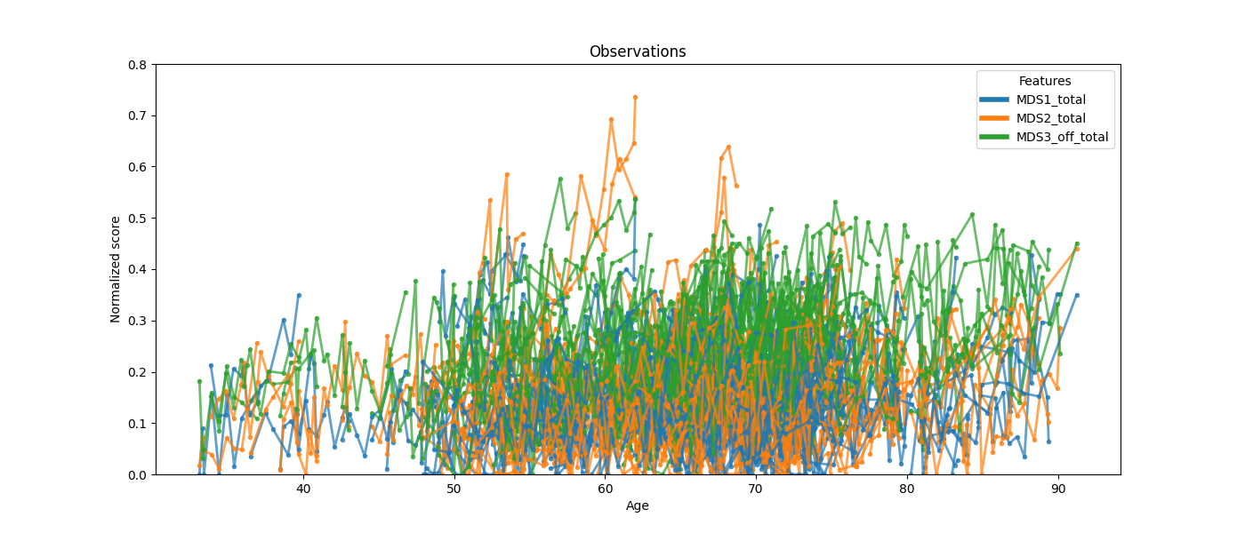
Raw training observations. The scores look heterogeneous because each patient is at a different disease stage and progresses at a different pace.
ax = leaspy_plotting.patient_observations(data_train, alpha=0.7, figsize=(14, 6))
ax.set_ylim(0, 0.8)
plt.show()
Fitting learns a single population-level sigmoidal curve that best explains all training subjects simultaneously.
model.fit(data_train, "mcmc_saem", seed=0, n_iter=100, progress_bar=False)
Fit with `AlgorithmName.FIT_MCMC_SAEM` took: 1.58s
The average trajectory is the shared progression curve. Every patient is assumed to follow this same curve, shifted and rescaled in time.
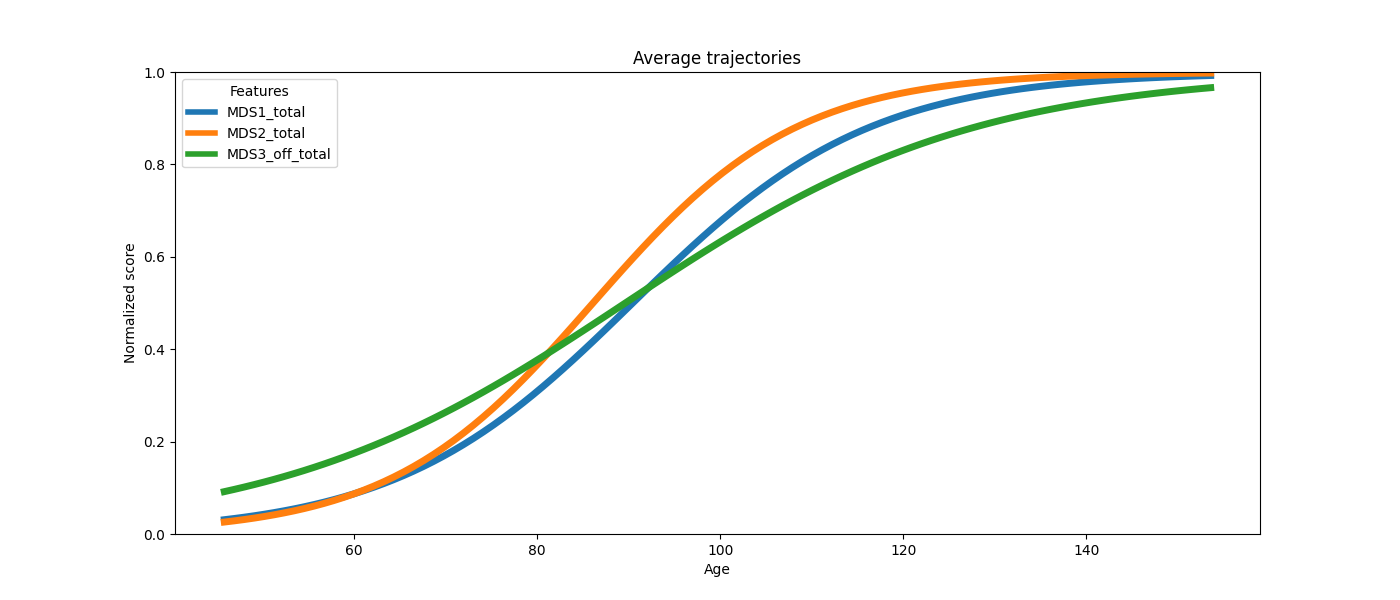
- Personalization estimates two individual parameters per test patient from their visits:
τ (tau) — disease onset age (position on the timeline) ξ (xi) — log-acceleration (pace of progression)
ip = model.personalize(data_test, "scipy_minimize", seed=0, progress_bar=False)
ip.to_dataframe().head()
Personalize with `AlgorithmName.PERSONALIZE_SCIPY_MINIMIZE` took: 13.02s
For example for the patient with ID GS-161 we observe a tau`of 57.69 and a xi of -0.29 (let’s ignore the sources parameters for the moment). To interpret the patient’s tau we should compare it with the population-level tau_mean.
model.parameters['tau_mean']
tensor([67.3562])
The average patient reaches the inflection point of the disease trajectory at age 67.35. The patient GS-161 has a tau of 57.69, which means that they are showing an earlier disease onset by approximately 10 years on the reparametrized disease timeline.
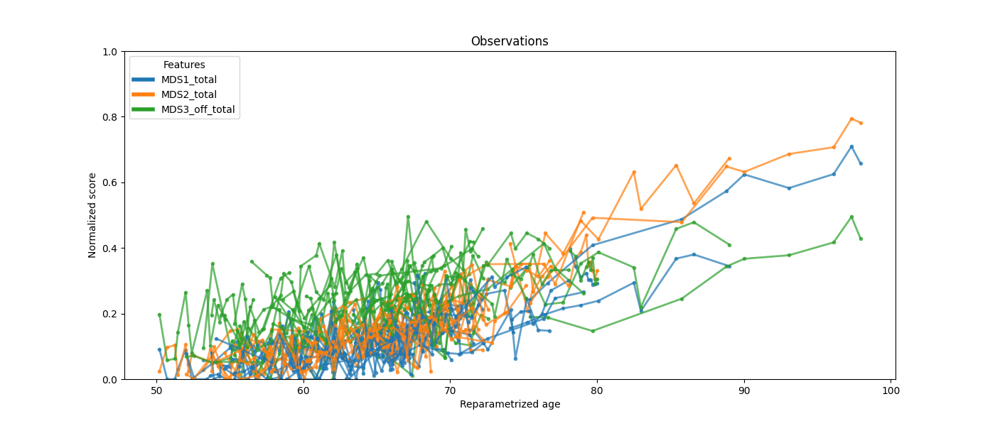
To interpret the patient’s xi we should compare it with 0. Patient GS-161 has a xi of -0.29, which means that they are progressing slower than the average patient, while patient GS-163 has a xi of 0.13 which means that they are progressing faster than the average patient. %% After time reparametrization ψᵢ(t) = exp(ξᵢ)·(t − τᵢ), all patients align onto the same curve — confirming the model has captured their individual stages and speeds.
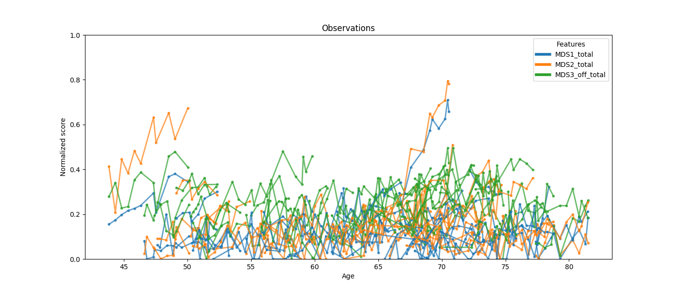
Without reparametrization the same data looks scattered: patients of the same chronological age may be at very different disease stages.
To illustrate prediction we pick one test patient. model.estimate is the low-level API that returns predicted scores at arbitrary timepoints — useful for custom analyses.
import numpy as np

print(f"Seen ages: {df_test.loc['GS-187'].index.values}")
print("Individual parameters:", ip["GS-187"])

timepoints = np.linspace(60, 100, 100)
reconstruction = model.estimate({"GS-187": timepoints}, ip)
print(f"Predicted scores at age 80: {reconstruction['GS-187'][40]}")  # index 40 ≈ age 80
Seen ages: [61.34811783 62.34811783 63.84811783 64.34812164 67.84812164 68.34812164
 69.34812164 69.84812164 70.84812164 71.34812164 71.84812164 72.34812164
 72.84812164 73.34812164]
Individual parameters: {'sources': [1.2316123247146606, 0.5551508665084839], 'tau': [73.25882720947266], 'xi': [0.06532679498195648]}
Predicted scores at age 80: [0.13828589 0.23553264 0.2740034 ]
patient_trajectories wraps that same call and overlays the predicted curve on the observed visits, extrapolating beyond the last observation.
ax = leaspy_plotting.patient_trajectories(
    data_test, ip,
    patients_idx=["GS-187"],
    labels=["MDS1", "MDS2", "MDS3 (off)"],
    figsize=(16, 6),
    factor_future=5,
)
ax.set_xlim(45, 120)
plt.show()
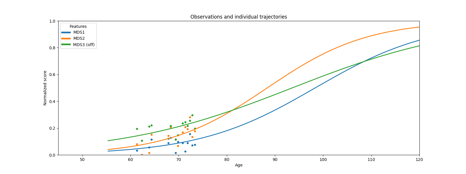
From a fitted model and just a few visits, Leaspy reduces each patient to (τ, ξ) — two numbers that place them on a shared disease timeline and predict their future trajectory across all scores simultaneously.
Interpreting the individual space shifts. Beyond (τᵢ, ξᵢ), each patient
also has a spatial signature — per-feature offsets that describe whether
they are more or less affected on certain features than the average
trajectory at tau_mean. These offsets are the
space shifts wᵢ,ₖ:
wᵢ,ₖhas one entry per feature, returned as columnsw_<feature>.A positive
w_MDS1for patient i means “given this patient’s (τ, ξ), they are more impaired on MDS1 than the average trajectory predicts”; negative means less impaired.By construction, the average
wᵢ,ₖis approximately zero.
ip.compute_space_shifts(model).head()
Large |wᵢ,ₖ| flags patients whose feature k is
atypically ahead or behind their overall stage — a signal worth a closer
look (alternative diagnosis, treatment response, comorbidity). This parameter
can be also interpreted “reverting” the features normalization, i.e. for the
MMSE that goes from 0 to 30, a wᵢ,MMSE = -0.1 means that patient i is 3
points better than the average patient at their stage.
The next example extends this to joint models that also incorporate time-to-event outcomes: see Joint Model.
Total running time of the script: (0 minutes 16.811 seconds)